Sound intensity, pressure, and decibels

Tags

Introduction

This page puts together information about several concepts of sound. I used and copied text, figures and tables from University Physics Volume 1 (Moebs et al, 2021) but also from some few other resources (including White and White, 2014) and the excellent website of Siemens.com that I refer to below. A such this page does not contain any new information and, in fact, there there are many other excellent (and better) resources about this topic. Nevertheless, by putting a selection of details together one a single page I hope this helps in understanding the relationship between sound intensity, sound pressure, and gain (in decibels).

Sound Intensity (I)

Energy (measured in Joules; $J$ ) is the ability to create a change, for example, creating motion. Power (measured in Watts; $W$ ) is how fast energy is used or transmitted – power is the amount of energy ( $J$ ) divided by the time ( $seconds$ ) it took to use the energy. One Watt is one joule per second of energy used ( $Watt = J \cdot s^{-1}$ )

Sound intensity is defined as the average time rate at which sound energy (Joules; $J$ ) passes through a unit area ( $A$ ) normal to the direction of the waves. It is an objective quantity associated with a sound wave. It can be measured, but not with a microphone. In contrast, loudness is a subjective response to the physical property of intensity depending on the condition of the hearing ability of an individual.

Sound intensity can also be defined as the time-averaged power per unit area ( $\langle P \rangle = W/m^2$ ) carried by a wave. Power is the rate at which energy ( $J$ ) is transferred by the wave (see also [here] for more background). Power is proportional to the square of the wave amplitude to the square of its angular frequency. For a spherical wave intensity $I$ is

$I = \frac{\langle P \rangle}{A} = \frac{\langle P \rangle}{4 \pi r^2}$

Power ( $J \cdot s^{-1}$ ) is defined as the transferred energy over a time period $T$ and therefore we can also write

$I = \frac{\langle E \rangle / T}{A}$

If there are no dissipative forces, the wave energy will remain constant as the spherical wave moves away from the source, but the intensity will decrease as the surface area increases. However, we usually express sound intensity as the power in Watt flowing through 1 square meter of area normal to the direction of the sound wave (White and White, 2014; Figure 1).

Figure 1. Sound intensity is defined as the power in Watt flowing through 1 square meter of area normal to the direction of the sound wave. Figure from White and White (2014).

Sound intensity level (L)

The range of intensities that the human ear can hear depends on the frequency of the sound, but the range is large. The minimum threshold intensity that can be heard is $I_0 = 10^{-12} W/m^2 = 1 pW/m^2$ (person with normal hearing at a frequency of 1.00 kHz). Pain is experienced at intensities of $I_{pain} = 1 W/m^2$ . Measurements of sound intensity in units of $W/m^2$ are cumbersome due to this large range in values. For this reason the concept of sound intensity level ( $L$ ) was proposed, which is a logarithmic scale. This is in agreement with the Weber-Fechner law that states that a response to any sense organ is approximately proportional to the logarithm of the magnitude of the stimulus.

The unit for intensity level is the bel (named for Alexander Graham Bell, the inventor of the telephone). However, this unit is seldom used, however, because the human ear is very sensitive. Humans can detect changes of as little as 1/10 of a bel, that is, a decibel. For that reason, sound intensity levels are defined in decibels (written as dB). The decibel is a relative unit, not an absolute one.

$L(dB) = 10 log_{10} \left( \frac{I}{I_0} \right)$

$I_0$ is the reference intensity.

How human ears perceive sound can be more accurately described by the logarithm of the intensity rather than directly by the intensity. Because $L$ is defined in terms of a ratio, it is a unitless quantity, telling you the level of the sound relative to the fixed reference. The units of decibels (dB) are used to indicate this ratio is multiplied by 10 in its definition.

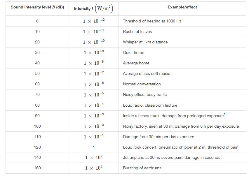
The decibel level of a sound having the threshold intensity of $10^{-12} W/m^2$ is $L = 0dB$ because $log_{10} (1) = 0$ . Table 1 gives levels in decibels and intensities in $W/m^2$ for some familiar sounds. From this table we see that each factor of 10 in intensity corresponds to 10 dB increase in sound intensity level. dB. For example, a 90-dB sound compared with a 60-dB sound is 30 dB greater, or three factors of 10 (that is 1000 times) as intense.

Table 1. Sound intensity level and sound intensity for some familiar sounds.

Changing Intensity Levels of a Sound

If we increase the intensity ( $I_1$ ) of a sound two-fold to $I_2$ then their ration is $\frac{I_2}{I_1} = 2$ . This difference in intensity results in a difference of sound intensity level equal to $L = 10 log_{10} \left( \frac{I_2}{I_1} \right) =10 log_{10} (2) = 3.01 dB$ . Note, that we effectively used $I_1$ as our reference level. This increase (gain) of sound level is true for any intensities that differ by a factor of two. Thus, a 56.0 dB sound is twice as intense as a 53 dB sound.

This is graphically shown in Figure 2 and Figure 3 which plot sound intensity vs sound intensity level.

Figure 2. Sound Intensity Level ( $L$ ; dB) vs Sound intensity ( $I$ ; $W/m^2$ ). On the x-axis the sound intensity ranges from $10^{-12} to 1 W/m^2$ . The range of the intensity level scale is much lower (from 0 to about 120dB).

Figure 3. Sound Intensity Level ( $L$ ; dB) vs $log_{10}$ Sound intensity ( $log_{10}(I)$ ; $W/m^2$ ). The x-axis values correspond to the exponents of the powers (i.e., $10^{exponent}$ ) that were plotted in Figure 1. The red lines indicate a two-fold increase of intensity from $10^{-10)$ to $2 \cdot 10^{-10)$ . The green lines indicate a two-fold increase of intensity from $10^{-2)$ to $2 \cdot 10^{-2)$ . In both cases the increase in level is 3.01dB.

Sound pressure level

Sound intensity is not the same physical quantity as sound pressure (measured in units of Pascal (Pa) or $N/m^2$ ) . Human hearing is sensitive to sound pressure which is related to sound intensity. In consumer audio electronics, the level differences are called “intensity” differences, but sound intensity is a specifically defined quantity and cannot be sensed by a simple microphone (wikipedia). Sound pressure can be measured in dB with a sound level meter.

The relation between Sound Intensity and Sound Pressure is given by

$\begin{align*} I = \frac{(\Delta p_{max})^2 }{2 \rho v} \end{align*}$

Here, $\Delta p_{max}$ is the pressure variation or pressure amplitude in units of pascals (Pa) or $N/m^2$ . $\rho$ is the density of the material in which the sound wave travels, in units of $kg/m^3$ , and $v$ is the speed of sound in the medium, in units of m/s.

Thus, we see that the sound intensity is related to the square of the pressure. This relationship is derived in the section ‘Relation of Sound Intensity and Pressure’ given below.

Due to this relationship we can write:

$\begin{align*} I(dB) &= 10 log_{10} \left( \frac{I}{I_0} \right) \\ &= 10 log_{10} \left( \frac{p^2}{p^2_0} \right) \\ &= \textbf{20} log_{10} \left( \frac{p}{p_0} \right) \end{align*}$

Thus, a doubling in sound pressure gives a change about about 6dB in sound intensity level (but better called Sound Pressure Level).

For example, if the pressure changes from 10 to 20 $N/m^2$ the the change in Sound Pressure Level is about 6dB. Since Sound Intensity is proportional to the square of the pressure, i.e., $I \sim p^2$ , we have a change in sound intensity of 100 to 200 which is also a two-fold increase. Hence, the sound intensity level changes about 3dB.

Since common microphones such as dynamic microphones produce a voltage ( $V$ ) which is proportional to the sound pressure (Figure 4), then changes in sound intensity incident on the microphone can be calculated from

$\begin{align*} I(dB) = 20 log_{10} \left( \frac{V_2}{V_1} \right) \end{align*}$

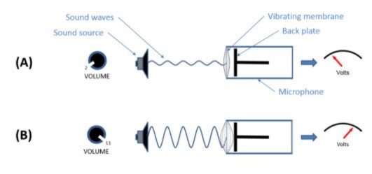
Figure 4. Translation op sound pressure into a voltage signal using a microphone. Figure copied from Siemens.com.

In general the formulation

$dB = \textbf{10} log_{10} \left( \frac{x}{x_{ref}} \right)$

is used for power quantities (like sound intensity) while the formulation

$dB = \textbf{20} log_{10} \left( \frac{x}{x_{ref}} \right)$

is used for amplitude quantities like pressure and voltage. The amplitude of field quantities (e.g. pressure, voltage) should be specified as root mean square (RMS) value.

Sound Intensity vs Sound Pressure

While sound pressure indicates the amplitude (Pa), it is a scalar quantity only (it does not indicate in which direction the sound is traveling). Sound intensity ( $W/m^2$ ) is vector quantity which indicates the flow of acoustic energy. Sound intensity has both a magnitude and direction (Siemens.com). Thus $\overrightarrow{I} = p(t) \times \overrightarrow{v}(t)$ .

Sound pressure, sound power, and sound intensity describe different aspects of sound but can all be expressed in terms of decibels (Table 2). A nice explanation of this quantity is by considering the analogy with a heater (see YouTube and Figure 5).

Table 2. Definition of sound pressure ( $p$ ), sound power ( $P$ ), and sound intensity ( $I$ ). Table copied from Siemens.com.

Figure 5. Heater analogy for Sound Pressure, Sound Intensity and Sound Power. Table copied from Siemens.com. The table is copied from Sengpiel audio.

Decibel Full Scale (dBFS)

Decibels relative to full scale (dBFS) is a unit of measurement for amplitude levels in digital systems such as pulse-code modulation (Wikipedia), and which is used in DAWs like Cubase. A level of 0 dBFS is assigned to the maximum possible digital level, thus all peak measurements smaller than the maximum are negative levels. For example, if a level reaches 50% of its maximum value then it has a level of -6dBFS (recall that $20 \cdot log_{10} \left( \frac{0.5}{1} \right) = -6dB$ .

The value in dBFS does not relate directly to the original absolute sound pressure level of the audio measured in dB.

The unit of dBFS is defined in several standards (e.g., AES17-2020, see also [here]) such that the Root Mean Square (RMS) value of a full-scale sine wave is designated 0dBFS. This implies that a full-scale square wave could have an RMS value of +3dBFS (see below).

The RMS value of a set of values (e.g., a continuous wave $f$ ) is the square root of the arithmetic mean of the squares of the values:

$x_{RMS} = \sqrt{\frac{1}{n} (x_1^2 + x_2^2 + \cdot \cdot \cdot + x_n^2) }$

For a continuous waveform $f(t)$ defined over an interval $T_1 \leq T \leq T_2$ the RMS can be defined as

$f_{RMS} = \sqrt{\frac{1}{T_2 - T_1} \int_{T_1}^{T_2} \left( f(t) \right)^2 \,dt$

For a sine wave with frequency $\omega=2 \pi f$ and amplitude $A=1$ , defined as $A sin(\omega t)$ over one period $T=\frac{2 \pi}{\omega}$ , the integral becomes

$f_{RMS} &= \sqrt{\frac{1}{2 \pi / \omega} \int_{t=0}^{2\pi / \omega} sin^2(\omega t) \,dt }$

Using the integration rule

$\int sin^2(a t) \,dt = \frac{t}{2} - \frac{1}{4a} sin(2at) +C$

This evaluates to

$\begin{align*} f_{RMS} &= \sqrt {\frac{1}{2 \pi / \omega} * \left( \frac{t}{2} - \frac{1}{4 \omega} sin (2 \omega t) \Bigr\rvert_{t=0}^{2 \pi / \omega} \right) } \\ &= \frac{1}{\sqrt{2}} \approx 0.7071 \end{align*}$

Thus, for a sinus wave with amplitude $A=1$ the RMS value = 0.7071. More general, if the amplitude = $A$ then $f_{RMS} = \frac{A}{\sqrt{2}}$ . Figure 6 shows the relation between amplitude and RMS.

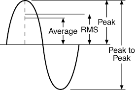
Figure 6. The relation between amplitude (peak), RMS, and average for a sinus wave. Figure copied from Quora.

Now we have defined RMS for a sinus wave we can return to dBFS. In standard IEC 61606-3 we find the following definitions:

Definition 3.4 dBFS. The RMS amplitude of a sinusoid described in 3.10 is defined as 0 dBFS, where the amplitude of any signal can be defined in dBFS as 20 times the common logarithm of the ratio of the RMS amplitude of the signal to that of the signal defined in 3.10.
Definition 3.10 Full scale amplitude. Amplitude of a 997 Hz sinusoid whose peak positive sample just reaches positive digital full-scale (in 2’s complement a binary value of 0111…1111 to make up the word length) and whose peak negative sample just reaches a value one away from negative digital full-scale (1000…0001 to make up the word length) leaving the maximum negative code (1000…0000) unused.

This definition implies that to determine dBFS the RMS of a signal is determined over a certain period of time. This definition would give us the following:

$dBFS = 20 log_{10} \frac{\text{RMS of signal}}{A_{max}}$

However, since the RMS of a full scale sinusoid is smaller than $A_{max}$ we need to correct for this:

$\begin{align*} dBFS &= 20 log_{10} \frac{\sqrt{2} \cdot \text{RMS of signal}}{A_{max}} \\ \\ &= 20 log_{10} \frac{\text{RMS of signal}}{A_{max}} + 20 log_{10} (\sqrt{2}) \\ \\ &= 20 log_{10} \frac{\text{RMS of signal}}{A_{max}} + 3.01 \end{align*}$

Thus, to show dBFS on a audio meter there is always a correction of +3.01 dB even if the signal is not a sinusoid. This implies that for non-sinusoid waves the dBFS may show positive values. For example, the RMS of a full-scale square wave = $A_{max}$ . Thus this gives:

$\begin{align*} dBFS &= 20 log_{10} \frac{\text{RMS of signal}}{A_{max}} + 3.01 \\ \\ &= 20 log_{10} \frac{A_{max}}{A_{max}} + 3.01 \\ \\ &=+3.01 \end{align*}$

This should also make clear that there are other ways to (incorrectly) implement dBFS. See for example [here]. I also tested dbFS in Cubase. Using it’s test generator, I generated a -3dB sinus (Figure 7) and a square (Figure 8) wave of 997 Hz. Interestingly, The Cubase +6dB Digital Scale meter shows an output of -3dBFS for the square wave while 0 dBFS was expected. The Waves Dorrough meter does show the correct levels.

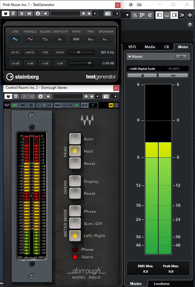
Figure 7. Test signal: -3dB sinus wave of 997 Hz. The Cubase meter (right) correctly shows a peak of -3dBFS dBFS and a RMS (end of green region) of -6dBFS (although I don’t understand why it says RMS Max = 0.0 dBFS). The Waves Dorrough meter only shows the peak level correctly at -3dBFS.

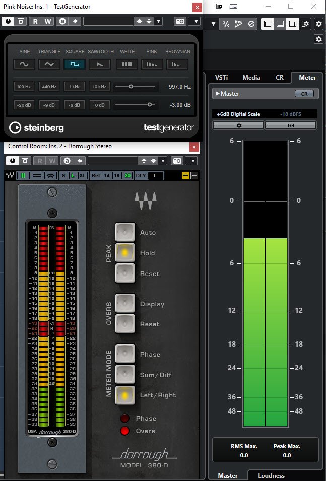
Figure 8. Test signal: -3dB square wave of 997 Hz. The Cubase meter (right) now correctly shows an RMS level (green region) of -6dBFS but the peak level did not increase to 0dBFS but also shows -3dBFS. Thus, Cubase does not seam to follow the standards precisely. However, it is correct in the sense that for a square wave the peak and RMS value are identical and are indeed -3dBFS. The Waves Dorrough meter only shows the peak level and, according to the standards, now correctly displays 0dBFS.

Note that dBFS is not defined for analog levels and depends on the standard chosen. For example 0VU (+4dBu) depends on the standard referred to (Figure 9):

-20 dBFS is the Digital AES reference standard.
-18 dBFS is the Digital EBU reference standard.
-14 dBFS is commonly used in post-production and certain mastering situations

Figure 9. Analog and digital audio levels. Figure copied from ZedBrookes.

Perception of loudness

A doubling of sound pressure (i.e., 6dB) is not perceived twice as loud by the human ear. Instead, a 10 dB increase (corresponding to a 3.16 fold-change in pressure) is perceived twice-as loud.

Relation of Sound Intensity and Pressure

In this rather lengthy section it is shown how sound intensity relates to pressure.

The intensity of a sound wave is proportional to the change in the pressure squared ( $p^2$ ) and inversely proportional to the density ( $\rho$ ) and the speed ( $v$ ). Note that I will use a small $p$ for pressure and a large $P$ for power. Consider a parcel of a medium initially undisturbed and then influenced by a sound wave at time $t$ , as shown in Figure 10:

Figure 10. An undisturbed parcel of a medium with a volume $V=A \Delta x$ shown in blue. A sound wave moves through the medium at time $t$ , and the parcel is displaced and expands, as shown by dotted lines. The change in volume is $\Delta V = A \Delta s = A (s_2 - s_1)$ , where $s1$ is the displacement of the leading edge of the parcel and $s2$ is the displacement of the trailing edge of the parcel. In the figure, $s2>s1$ and the parcel expands, but the parcel can either expand or compress ( $s2<s1$ ), depending on which part of the sound wave (compression or rarefaction) is moving through the parcel.

As the sound wave moves through the parcel, the parcel is displaced and may expand or contract. The change in the volume is

$\Delta V = A \Delta s = A(s2-s1) = A \left( s(x+\Delta x,t) - s(x,t) \right)$

The fractional change in the volume is the change in the volume divided by the original volume:

$\frac{\Delta V}{V} = \lim_{ \Delta x \rightarrow 0 } \frac{A \left( s(x+\Delta x,t) - s(x,t) \right)}{A \Delta x} = \frac{\delta s(x,t)}{\delta x}$

The fractional change in volume is related to the pressure fluctuation by the bulk modulus $\beta = - \frac{\Delta p(x,t)}{dV/V}$ . Thus, the change in pressure is

$\Delta p(x,t) = - \beta \frac{dV}{V} = -\frac{\delta s(x,t)}{\delta x}$

If the sound wave is sinusoidal then the displacement is $s(x,t) = s_{max} cos(kx \mp \omega t + \phi)$ (see [here]) with the minus sign to indicate the positive x-direction. Then the pressure is

$\Delta p(x,t) = - \beta \frac{\delta s(x,t)}{\delta x} = - \beta \frac{\delta}{\delta x} s_{max} cos(kx - \omega t + \phi) = \beta k s_{max} sin(kx - \omega t + \phi) = \Delta p_{max} sin(kx - \omega t + \phi)$

Note that the derivative of cos is -sin.

Since intensity ( $I$ ) of the sound wave is the power per unit area ( $\frac{P}{A}$ ), power is the force ( $F$ ) times velocity ( $v$ ), and pressure ( $p$ ) is the force applied perpendicular to the surface of an object per unit area, we derive that intensity is:

$I = \frac{P}{A} = \frac{F v }{A} = pv$

Note, that the velocity $v$ is the velocity of the oscillations of particles in the medium, and not the velocity of the $v$ . The velocity of the medium is:

$v(x,t) = \frac{\delta}{\delta t} s(x,t) = \frac{\delta}{\delta t} s_{max} cos(kx - \omega t + \phi) = s_{max} \omega sin(kx - \omega t + \phi)$

Thus, this gives the following equation for the intensity:

$\begin{align*} I &= \Delta P(x,t) v(x,t) \\ &= \beta k s_{max} sin(kx - \omega t + \phi) \times s_{max} \omega sin(kx - \omega t + \phi) \\ &= \beta k \omega s^{2}_{max} sin^{2}(kx - \omega t + \phi) \end{align}$

To find the time-averaged intensity over one period $T = \frac{2 \pi}{\omega}$ for a position $x$ we need to integrate over one period and divide by the period:

$ = \frac{1}{T} \int_{0}^{T= \frac{2 \pi}{\omega}} \beta k \omega s^{2}_{max} sin^{2}(kx - \omega t + \phi) \,dt$

To integrate this function we can use the cos double angle formula $cos(2x) = 1 - 2 sin^{2} (x) \rightarrow sin^{2} (x) = \frac{1}{2} (1 - cos(2x)$ . We get:

$\begin{align*} &= \frac{1}{2T} \beta k \omega s^{2}_{max} \int_{0}^{\frac{2 \pi}{\omega}} \left( 1 - cos(2kx - 2 \omega t + 2 \phi ) \right) \, dt \\ &=\frac{1}{2T} \beta k \omega s^{2}_{max} \int_{0}^{\frac{2 \pi}{\omega}} \,dt -\frac{1}{2T} \beta k \omega s^{2}_{max} \int_{0}^{\frac{2 \pi}{\omega}} cos(2kx - 2 \omega t + 2 \phi ) \, dt \end{align*}$

First solve the first integral

$\frac{1}{2T} \beta k \omega s^{2}_{max} \int_{0}^{\frac{2 \pi}{\omega}} \,dt$

Using $T=\frac{2 \pi}{\omega} \rightarrow \omega = \frac{2 \pi}{T}$ , this gives

(1) $\begin{equation*} \begin{split} \frac{1}{2T} \beta k \omega s^{2}_{max} t \Bigr\rvert_{t=0}^{t=2 \pi / \omega} \\ \\ \rightarrow \frac{1}{2T} \beta k \omega s^{2}_{max} \frac{2 \pi}{\omega} - 0 \\ = \beta k \omega s^{2}_{max} \frac{2 \pi}{2 T \omega} = \frac{\pi}{T} \frac{1}{\omega} \\ \\ = \beta k \omega s^{2}_{max}\frac{\pi}{T} \times \frac{T}{2 \pi} = \frac{\beta k \omega s^{2}_{max}}{2} \end{split} \end{equation*}$

To solve the second integral we change the integration variable

$\begin{align*} u = 2(kx -\omega t + \phi) \\ \frac{du}{dt} = - 2 \omega \\ dt = \frac{du}{2 \omega} \end{align*}$

This gives

$\begin{align*} I &= -\frac{1}{2T} \beta k \omega s^{2}_{max} \int_{0}^{\frac{2 \pi}{\omega}} cos(2kx - 2 \omega t + 2 \phi ) \, dt \\ &= -\frac{1}{2T} \beta k \omega s^{2}_{max} \int_{0}^{\frac{2 \pi}{\omega}} \frac{cos(u)}{2 \omega} \, du \\ & = \frac{1}{2 \omega} \beta k \omega s^{2}_{max} sin(u) \end{align*}$

Back substitution of $u$ and doing the algebra, this expression evaluates to 0.

Thus, together, the integral

$ = \frac{1}{T} \int_{0}^{T= \frac{2 \pi}{\omega}} \beta k \omega s^{2}_{max} sin^{2}(kx - \omega t + \phi) \,dt$

evaluates to the time averaged intensity

$ = \frac{\beta k \omega s^{2}_{max}}{2}$

Multiplying with $\frac{\beta k}{\beta k}$ gives

$ = \frac{\beta^2 k^2 \omega s^{2}_{max}}{2 \beta k}$

Using $\Delta p_{max} = \beta k s_{max}$ gives

$ = \frac{(\Delta p_{max})^2 \omega}{2 \beta k}$

Using $v = \frac{\omega}{k}$ gives

$ = \frac{(\Delta p_{max})^2 v}{2 \beta}$

Using $v = \sqrt \frac{\beta}{\rho} \rightarrow \beta = v^2 \rho$ gives

$\begin{align*} &= \frac{(\Delta p_{max})^2 v}{2 v^2 \rho} \\ &= \frac{(\Delta p_{max})^2 }{2 \rho v} \end{align*}$

Thus, we see that the sound intensity is related to the square of the pressure.

References

Moebs W, Ling, SJ, Sanny J (2021) University Physics Volume 1. Web version January 19, 2021. Openstax, Houston. https://openstax.org/details/books/university-physics-volume-1. This book is licensed under Creative Commons Attribution License v4.0
White HE, White DH (2014) Physics and Music. The Science of Musical Sound, Dover Publications, Mineola.
The Wacky World of Acoustics (Siemens)

University Physics Volume 1 (chapter 15-17) (pdf)

1 file(s) 14.57 MB

Download

dB or not dB (pdf)

1 file(s) 1.09 MB

Download

Published On: July 14th, 2021Last Updated: January 3rd, 2024Categories: Audio technology EducationTags: audio technology, decibels, sound intensity, sound pressure, sound waves

Cookie	Duration	Description
cookielawinfo-checkbox-analytics	11 months	This cookie is set by GDPR Cookie Consent plugin. The cookie is used to store the user consent for the cookies in the category "Analytics".
cookielawinfo-checkbox-functional	11 months	The cookie is set by GDPR cookie consent to record the user consent for the cookies in the category "Functional".
cookielawinfo-checkbox-necessary	11 months	This cookie is set by GDPR Cookie Consent plugin. The cookies is used to store the user consent for the cookies in the category "Necessary".
cookielawinfo-checkbox-others	11 months	This cookie is set by GDPR Cookie Consent plugin. The cookie is used to store the user consent for the cookies in the category "Other.
cookielawinfo-checkbox-performance	11 months	This cookie is set by GDPR Cookie Consent plugin. The cookie is used to store the user consent for the cookies in the category "Performance".
viewed_cookie_policy	11 months	The cookie is set by the GDPR Cookie Consent plugin and is used to store whether or not user has consented to the use of cookies. It does not store any personal data.

Music, composing, mixing, and mastering

Sound intensity, pressure, and decibels

University Physics Volume 1 (chapter 15-17) (pdf)

dB or not dB (pdf)

Leave A Comment Cancel reply

Sound intensity, pressure, and decibels

University Physics Volume 1 (chapter 15-17) (pdf)

dB or not dB (pdf)

Leave A Comment Cancel reply

Related Posts

Mixclub ’22 – Anniversary

Why you do not need Thunderbolt for professional audio (by RME Audio)

Know your microphone

From frequency to wavelength