![]()

| Recent Comments |
| Categories |
| Archives |
| Tags |
From (True) Peak via RMS to LUFS
Introduction to Decibels: What is a dB?
For a more detailed description see my posts on Decibels. The intensity of a sound wave is the average amount of energy transmitted per unit time through a unit area in a specified direction. The amount of energy per unit time is power, and intensity is therefore the amount of power transmitted through a unit area in a specified direction. Power is measured in watts, and intensity is therefore measured in watts per square meter.
Scientists often specify sound intensity as a ratio, however. The sound intensity level, I, in decibels is defined as 10 times the logarithm of the ratio of the intensity of a sound wave to a reference intensity:

The unit for intensity is the bel. However, this unit is seldom used, however, because the human ear is very sensitive. Humans can detect changes of as little as 1/10 of a bel, that is, a decibel. For that reason, sound intensity levels are defined in decibels (written as dB). The decibel is a relative unit, not an absolute one.
Acoustic intensity is rarely measured directly, however. Microphones measure the pressure (amplitude) of a sound wave rather than its intensity. Because the intensity of a sound wave is proportional to the square of its pressure p:
![]() (“ρ” is the density of medium carrying the sound and c is the speed of sound), the sound pressure level in dB can be computed directly from the measured pressure:
(“ρ” is the density of medium carrying the sound and c is the speed of sound), the sound pressure level in dB can be computed directly from the measured pressure:
![]()
To be able to compare sound levels given in dB to one another, a standard reference intensity or reference pressure must always be used. In air, however, scientists have agreed to use the intensity of a sound wave with a pressure of 20 microPascals as the reference intensity.
The logarithmic nature of the dB scale means that each 10 dB increase is a ten-fold increase in acoustic power. A 20-dB increase is then a 100-fold increase in power, and a 30-dB increase is a 1000-fold increase in power. A ten-fold increase in acoustic power does not mean that the sound is perceived as being ten times louder, however. Humans perceive a 10 dB increase in sound level as only a doubling of sound loudness, and a 10 dB decrease in sound level as a halving of sound loudness.
Audio Levels in the analog and digital domain
The basic DAW (e.g., Cubase) shows the (true) peak level corresponding with +24dBu in the analog domain. The normal operating level in the analog domain is +4dBU corresponding to 0VU on a VU meter. This gives 20db of head room in analog systems. Consequently, it is recommended to use the same amount of head room in digital systems. See my K-20 calibration. Figure from Sound On Sound.

Note that the correspondence with 0VU (+4dBu) depends on the standard referred to:
- -20 dBFS is the Digital AES reference standard.
- -18 dBFS is the Digital EBU reference standard.
- -14 dBFS is commonly used in post-production and certain mastering situations
A similar figure comes from Zed Brooks in an article about recording levels:

(True) Peaks
The True Peak meter algorithm recognises inter-sample peaks which are often missed by the simple sample-peak meters typically provided in DAW software such as Cubase. Sample-peak meters display only the highest amplitude value of a group of consecutive samples, and the scale is calibrated in dBFS (decibels below full scale), with 0dBFS at the top. To differentiate a True Peak meter reading from a conventional sample-peak meter, the new scale is marked in dBTP (decibels, true peak), and typically goes up to +3 or +6dBTP. Figure below from Sound On Sound. See also the discussion and video on gearspace.com for some discussion.

RMS – Root mean square
In mathematics and its applications, the root mean square (RMS) is defined as the square root of the mean square (the arithmetic mean of the squares of a set of numbers). RMS is nicely explained [here] and [here].
The following figure shows the three most common ways of characterizing the loudness of a sound signal. The two simplest ways of characterizing a sound wave are by its peak pressure and by its peak-to-peak pressure. The peak pressure, also called the 0-to-peak pressure, is the range in pressure between zero and the greatest pressure of the signal. The peak-to-peak pressure is the range in pressure between the most negative pressure and the most positive pressure of the signal. A more complex way of characterizing a sound wave is the root-mean-square pressure. The root-mean-square pressure (abbreviated as RMS pressure) is the square root of the average of the square of the pressure of the sound signal over a given duration.

The root-mean-square pressure is most often used to characterize a sound wave because it is directly related to the energy carried by the sound wave, which is called the intensity. The intensity of a sound wave is the average amount of energy transmitted per unit time through a unit area in a specified direction. The intensity I of a sound wave is proportional to the average over time of the square of its pressure p (See Introduction to Decibels):
![]()
The density and sound speed are relatively constant, and so the intensity is directly related to the mean square pressure:
![]()
The root-mean-square (rms) pressure is then just the square root of this:
![]()
The R<S pressure is most often used to characterize sound waves that have the simple shape shown in the above figure. Not all sound waves have such simple shapes, which contain only one frequency. The situation becomes more complicated when the sound signal is a short impulsive signal, such as sound waves generated by a snare drum. It is easy to estimate the peak-to-peak and peak pressures in these cases, but it becomes more difficult to calculate the RMS pressure.
The RMS method requires the scientist to select a duration over which to average the pressure of the signal. This method is appropriate for tones in which the average pressure can be directly related to the intensity of the sound signal. It is not appropriate to use RMS pressure to measure impulsive sounds, since the RMS pressure will vary dramatically depending on the duration over which the signal is averaged. In fact, the longer the time duration over which the signal is averaged, the lower the RMS value will be. This is illustrated in the following figure, where the RMS pressure is calculated using three different durations for an impulsive signal.

Loudness War
The current trend is all about trying to make a CD or download sound as loud as possible compared with other commercial material. Yet listening loudness is easily determined by the user via the volume control. The key to Katz’s claim is an ongoing industry shift into a ‘loudness normalisation realm’, in which the replay level of individual tracks is adjusted automatically to ensure they all have the same overall perceived loudness. Within a loudness-normalisation environment, it becomes impossible to make any one track appear to sound louder, overall, than any other, so mastering to maximise loudness inherently becomes completely futile.
In the all-analogue days, mixing consoles, tape machines, vinyl discs and other consumer replay media all employed a nominal ‘reference level’, essentially the average programme signal level. Above this reference level, an unmetered space called ‘headroom’ was able to accommodate musical peaks without clipping. This arrangement allowed different material to be recorded and played with similar average loudness levels, whilst retaining the ability to accommodate musical dynamics too. With the move into digital audio, the converters in early CD mastering and playback systems weren’t as good as they really should have been, and to maximise audio quality, the signal levels had to peak close to 0dBFS (ie. the maximum digital peak level). Consequently, the ‘reference level’ effectively became the clipping level, and the notion of headroom fell by the wayside.
The typical way that a track is made to sound loud on a CD is by employing heavy limiting and compression to increase the average energy level and minimise the crest factor, or peak-to-average ratio. This squeezes much of the audio signal up towards the digital system’s maximum peak level.
A very interesting article from Sound On Sound demonstrates how compression (to get louder) affects an audio file.
Perceived loudness
Perceived loudness is essentially based on the average energy level of a track; the higher the average energy level, the louder the track will sound. The technical term is ‘peak normalisation’: raising the level of the signal so that its peaks hit a defined maximum level. The flip side of this coin is that we lose the headroom margin, so there is no longer any room for musical dynamics. We can’t raise the peak level any further, only the average level through compression/limiting.
An important fact to note about loudness normalisation is that it is nothing more than a static volume adjustment for each programme, based on an assessment of the programme’s qualitative loudness level, measured over its full duration. That last point is important. The loudness value is determined across the whole programme duration, whether it’s a 30-second commercial or a two-hour feature film, and not moment to moment. Once the loudness value is determined, the replay level can be adjusted for that programme or advert, so that its loudness conforms to the defined ‘target loudness level’.
Loudness normalisation just does what most listeners do instinctively with their remote control; it adjusts the replay level to a comfortable volume and maintains that automatically between different programmes or channels.
Algorithms to measure Audio Programme Loudness and True Peak Audio Level
The loudness-metering algorithm (basically an electronic ear) involves 4 stages (Figure below from SoundOnSound):
- Response filtering
- Average-power calculation
- Channel weighting
- Summation (integration over 400ms).
- Logarithmic conversion and integration (calculation average over complete audio file)

The response filtering stage is called ‘K-weighting’ and it combines a boosting high-shelf equaliser with a high-pass filter (Figure below from Mathworks.com; also show A and C weighting) . The shelf equaliser provides 4dB boost above about 2kHz and is intended to replicate the acoustic effects of the head (see also here). The high-pass filter simulates our reduced sensitivity to low frequencies when it comes to assessing loudness, with a 12dB/octave filter turning over at roughly 100Hz.

The next stage determines the average signal power using a mean-square calculation (ie. the average of the squared values of sample amplitudes). The power is averaged over a 400ms measuring period which is updated every 100ms. Note: a VU meter integrates over 300ms and gives a more rough estimate of perceived loudness.
Following this channel summation, the loudness value is given as a logarithmically scaled number in Loudness Units relative to digital full scale (LUFS) —so it will always be a negative number. Where a relative (rather than absolute) loudness scale is more appropriate or
convenient, the deviation in loudness from a given Target Loudness level can be given in Loudness Units (LU). For example, if the target level is -23LUFS but the material actually measures -20LUFS, its loudness offset would be described as +3LU.
Although the basic principles of the loudness algorithm are fairly straightforward, there’s some added complexity to make sure that quiet periods don’t drag the average loudness value down unfairly. For a start, if the signal level lies below -70LUFS it plays no part in the loudness measurement process. This makes sure that silent sections at the start and end of a programme don’t affect the loudness value. Secondly, if the audio level falls 10dB below the current programme loudness
The latest version can be retrieved from the ITU website.
Loudness and true-peak audio level (Recommendation ITU-R BS.1770-4) (pdf) 955.36 KB 359 downloads
Algorithms to measure audio programme loudness and true-peak audio level (Recommendation...
Many more details about loudness measurement and normalization can be found in this master thesis:
Adaptive Normalisation of Programme Loudness in Audiovisual Broadcasts (MSc thesis) (pdf) 1.19 MB 305 downloads
Herman Molinder (2016) Adaptive Normalisation of Programme Loudness in Audiovisual...
Update of loudness standard (2021). AES TD1008.1.21-9. Recommendations for Loudness of Internet Audio Streaming and On-Demand Distribution
Loudness meters
In addition to the Integrated Loudness value, most loudness meters display five other parameters. The first two are usually labelled M and S. The M value is ‘Momentary’ and based on a sliding 400ms window updated every 100ms, so that it gives an indication of the instantaneous loudness. This is intended to aid initial level-setting when starting a mix, and in many meters the M value is displayed as a bar-graph, where it behaves in a very similar way to a standard VU meter. The S value is the ‘Short-Term’ or ‘Sliding’ loudness value, which is based on a sliding three-second window. When mixing material on the fly, the S value is the one to keep an eye on as it responds reasonably quickly to mixing adjustments and provides a good indication of where the mix loudness is in relation to the target value, moment to moment.
Below the loudness meters in Cubase (top: Control Room; bottom: Supervision plugin).


Loudness normalisation by streaming services
Nowadays streaming services apply loudness normalisation when required. This normalisation will not change the sound of a mix but only its volume. In the table below you find the current Loudness targets for different streaming services.


Some tips from Mastering the Mix:
- Your music will get turned down if it’s louder than about -14 LUFS. Going for a more dynamic and punchy mix will sound better than an over-compressed, distorted master. For example, keep your music below -8 short-term LUFS during the loudest part of the song for Spotify.
- Spotify suggests leaving at least -1dBTP (decibels true peak) of headroom when submitting music so they are optimized for the lossy formats. They suggest -2dBTP of headroom for loud track, as loud tracks have a greater chance of clipping during transcoding. Spotify streams audio using Ogg Vorbis and AAC files which are almost guaranteed to increase the peak levels.
- Don’t master too quiet! Amazon music turns louder songs down, but doesn’t currently turn the quiet tracks up. You wouldn’t want your song to lack energy compared to the other tracks, so try to keep the overall integrated LUFS value at -16 LUFS or louder.
- Soundcloud is different when it comes to loudness. Soundcloud doesn’t normalize the volume playback on their tracks. But it’s worth noting that they transcode all their audio to 128kbps MP3 for streaming. When the track is transcoded, some clipping and distortion can take place. Louder tracks with higher peaks suffer the worst from the encoding and end up sounding crunchy and lacking clarity. Leave at least -1dBTP of headroom when mastering for Soundcloud and try not to go louder than -7 LUFS short-term.
Some additional notes on Z, A, and C-weighting

If a sound is produced with equal sound pressure across the whole frequency spectrum, it could be represented in the graph below by the Z-Weighting line. What humans are physically capable of hearing is represented by the A-Weighting curve. Acoustic sound contains more lower and higher frequencies than humans perceive. The C-Weighting curve represents what humans hear when the sound is turned up; we become more sensitive to the lower frequencies. The A and C weightings are thus most meaningful for describing the frequency response of the human ear toward real world sounds. [NTI audio]
Note: Large part of the text was copied from the following references, which I fully acknowledge:
References
- To the Limit. Dynamic Range & Loudness War (Sound On Sound)
- The End of the Loudness War? The New Normal (Sound On Sound)
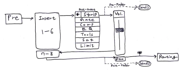
- Level headed. Gain staging in your DAW software (Sound On Sound)
- International Telecommunication Union (ITU)
- https://www.nti-audio.com/en/support/know-how/frequency-weightings-for-sound-level-measurements
- Adaptive Normalisation of Programme Loudness in Audiovisual Broadcasts (MSc Thesis, Herman Molinder)


